Adjustments to RPID for Scanning
Since RPID was already working and callable from Lab 8, I used it for orientation control. It fits naturally into the SCAN case, rotating the robot in fixed degree increments and stopping at each one while the sensors collect readings. Keeping the robot stationary for every measurement is important, as the ToF sensor can produce false outputs if the target distance is changing during integration.
I used 20 degree steps for 18 stops per full rotation, exceeding the 14 reading minimum. RPID settles within 2 degrees of each target, and since the integrator resets on every call, gyro drift does not accumulate as much across steps. For an on-axis turn in the center of a 4x4m empty room, a 2 degree angular error at 2m wall distance corresponds to roughly 40mm of positional error. At the maximum corner distance of approximately 2.83m this grows to around 78mm.
void RPID(float s) {
    float setpoint = s;
    float kp = 2.0f;
    float ki = 0.07f;
    int max_pwm = 60;
    int min_pwm = 45;

    float integral_error = 0.0f;
    float yaw_angle_deg  = 0.0f;
    float gyro_z_bias    = 0.0f;

    for (int i = 0; i < 2; i++) {
        myICM.getAGMT();
        gyro_z_bias += myICM.gyrZ();
    }
    gyro_z_bias /= 2.0f;

    unsigned long last_control_us = micros();
    float error = setpoint;

    while (fabs(error) > 1.0f) {
        myICM.getAGMT();
        unsigned long now_us = micros();
        float dt_control = (now_us - last_control_us) / 1000000.0f;
        if (dt_control <= 0.0f) continue;
        last_control_us = now_us;

        float gyro_z_dps = myICM.gyrZ() - gyro_z_bias;
        yaw_angle_deg += gyro_z_dps * dt_control;
        error = setpoint - yaw_angle_deg;

        integral_error += error * dt_control;
        if (integral_error >  100.0f) integral_error =  100.0f;
        if (integral_error < -100.0f) integral_error = -100.0f;

        float control = kp * error + ki * integral_error;
        int pwm_val = 0;

        if (fabs(error) < 2.0f) {
            car.kill();
            break;
        } else {
            pwm_val = (int)fabs(control);
            if (pwm_val < min_pwm) pwm_val = min_pwm;
            if (pwm_val > max_pwm) pwm_val = max_pwm;
        }

        if (error > 0.0f) { car.tl(pwm_val); }
        else              { car.tr(pwm_val); }
    }
    car.kill();
}
My SCAN Case
The SCAN case takes four BLE arguments: number of steps, degrees per step, and x and y coordinates. The coordinates are logged in every transmitted data line so the Python notification handler can sort readings by position automatically. At each stop a 100ms delay allows both sensors to settle, then 4 readings from each ToF are averaged before RPID rotates to the next step. Step count and increment are configurable from Python without modifying the Arduino code.
Scans were collected at five positions. Because the robot was started at a 90 degree offset from the intended orientation, the x and y coordinate inputs are swapped and sign-flipped relative to the lab specification. The transformation matrices account for this correctly as long as the coordinates are entered consistently.
case SCAN: {
    int steps = 12;
    int deg_per_step = 30;
    float x_pos = 0.0f;
    float y_pos = 0.0f;

    if (!robot_cmd.get_next_value(steps))        break;
    if (!robot_cmd.get_next_value(deg_per_step)) break;
    if (!robot_cmd.get_next_value(x_pos))        break;
    if (!robot_cmd.get_next_value(y_pos))        break;

    float scan_tof1_array[steps];
    float scan_tof2_array[steps];
    float scan_yaw_array[steps];
    float cumulative_yaw = 0.0f;

    tof1.startRanging();
    tof2.startRanging();

    for (int step = 0; step < steps; step++) {

        delay(100); // settle time before measuring

        float sum1 = 0.0f, sum2 = 0.0f;
        int count1 = 0, count2 = 0;

        while (count1 < 4 || count2 < 4) {
            if (count1 < 4 && tof1.checkForDataReady()) {
                sum1 += tof1.getDistance();
                tof1.clearInterrupt();
                count1++;
            }
            if (count2 < 4 && tof2.checkForDataReady()) {
                sum2 += tof2.getDistance();
                tof2.clearInterrupt();
                count2++;
            }
        }

        scan_tof1_array[step] = sum1 / 4.0f;
        scan_tof2_array[step] = sum2 / 4.0f;
        scan_yaw_array[step]  = cumulative_yaw;

        if (step < steps - 1) {
            tof1.stopRanging();
            tof2.stopRanging();
            RPID((float)deg_per_step);
            cumulative_yaw += (float)deg_per_step;
            tof1.startRanging();
            tof2.startRanging();
        }
    }

    car.kill();
    tof1.stopRanging();
    tof2.stopRanging();

    for (int i = 0; i < steps; i++) {
        tx_estring_value.clear();
        tx_estring_value.append("SCAN:");
        tx_estring_value.append(x_pos);      tx_estring_value.append(",");
        tx_estring_value.append(y_pos);      tx_estring_value.append(",");
        tx_estring_value.append(scan_yaw_array[i]);  tx_estring_value.append(",");
        tx_estring_value.append(scan_tof1_array[i]); tx_estring_value.append(",");
        tx_estring_value.append(scan_tof2_array[i]);
        tx_characteristic_string.writeValue(tx_estring_value.c_str());
        delay(10);
    }

    break;
}
Demo
The video below shows the SCAN case running at position (2, -3) in my reference frame, which corresponds to (-3, -2) in the lab reference frame.
Transformation Matrices
To merge all scan positions into a single world frame map, a transformation matrix T was computed for each position encoding the robot's location (x, y) and heading theta. Multiplying a robot-frame point by T gives its world frame coordinates.
The front ToF (tof1) is 75mm from center along robot y, and the side ToF (tof2) is 30mm from center along the negative robot x axis. A tof1 reading of distance d maps to (0, 75+d) and a tof2 reading of distance d maps to (-(30+d), 0) in robot frame. Robot positions are specified in feet and converted to mm before the transform is applied.
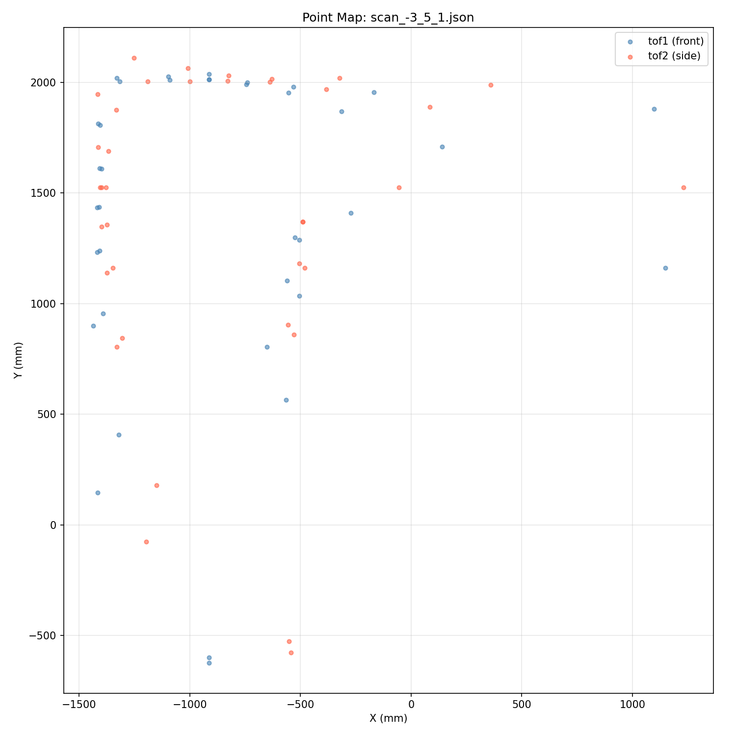
Scan Results
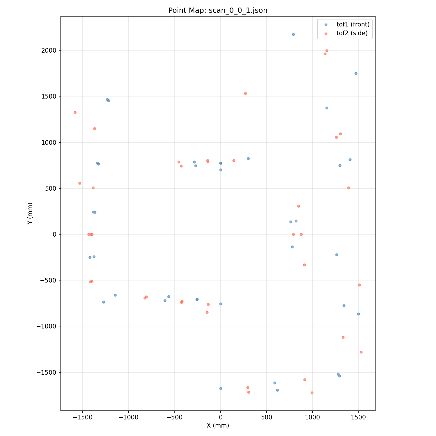
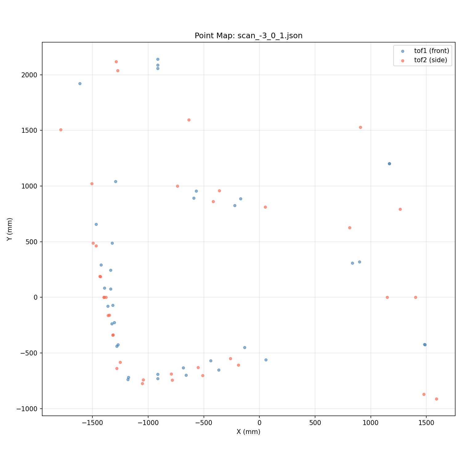
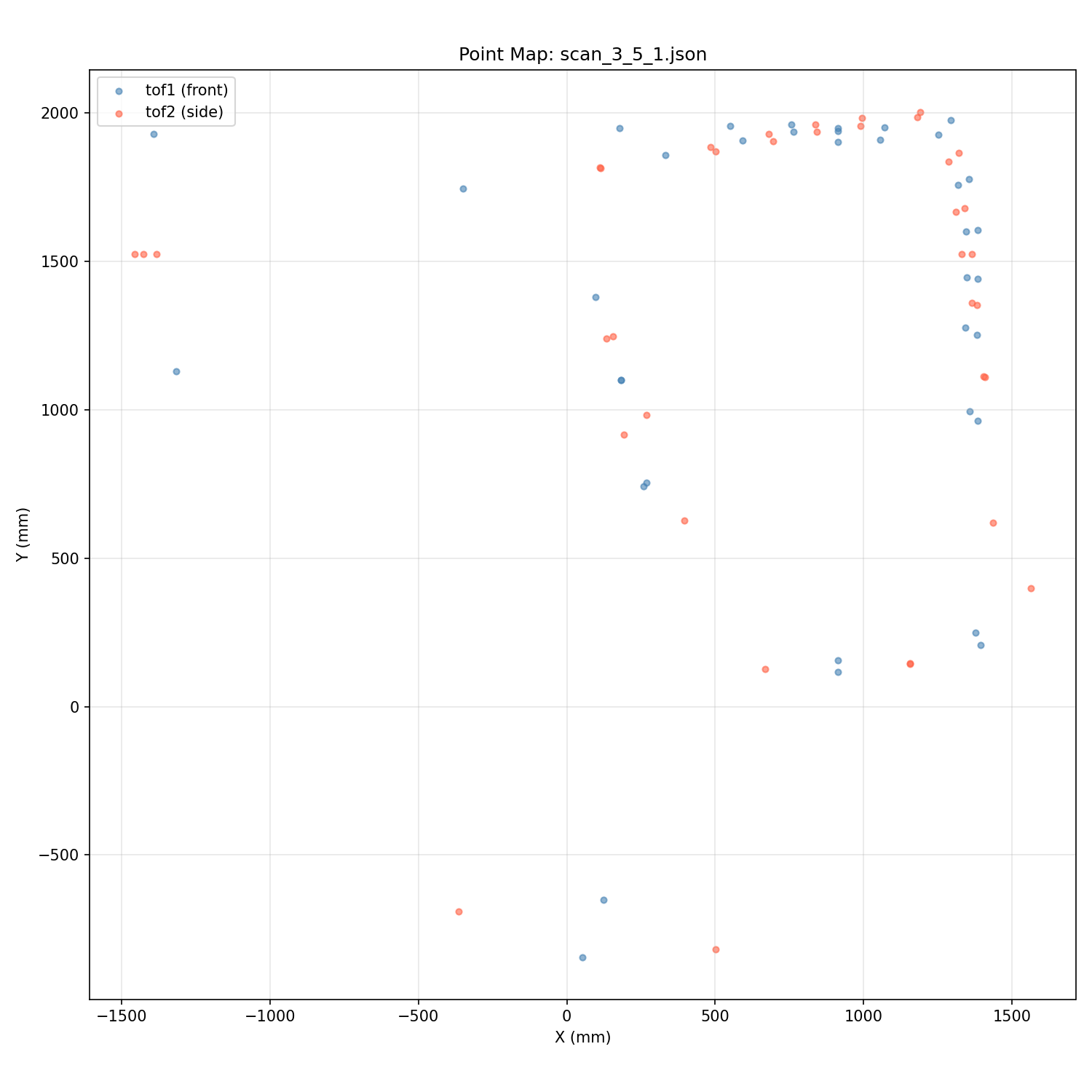
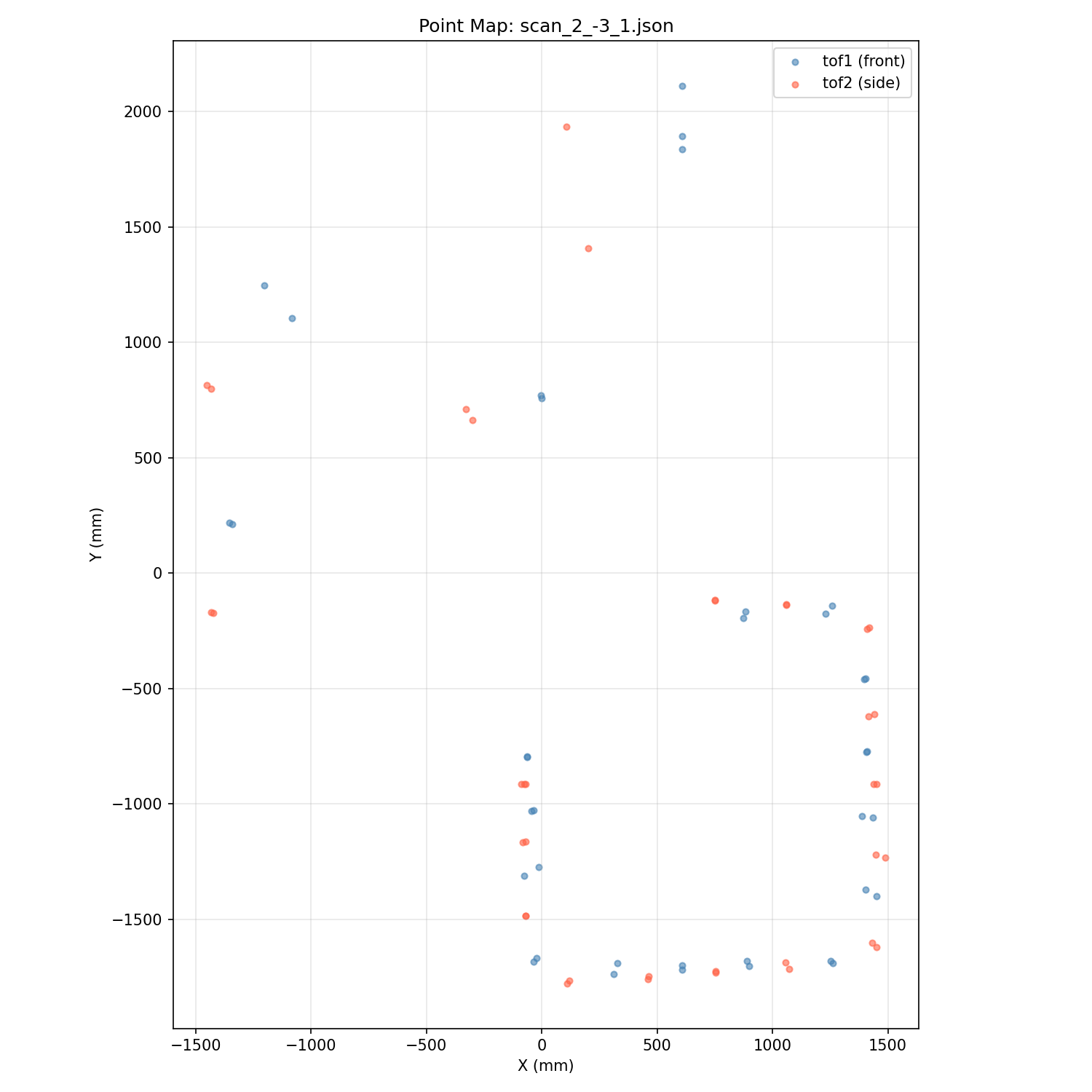
The five scan positions in my reference frame were (-3, 0), (-3, 5), (0, 0), (2, -3), and (3, 5), corresponding to the lab spec positions with swapped and sign-flipped coordinates due to the 90 degree starting offset described above.
Individual Scan Plots
Each scan is plotted in polar coordinates from the robot's position as a sanity check. The shapes are consistent with the expected lab geometry at each location.
Combined World Map
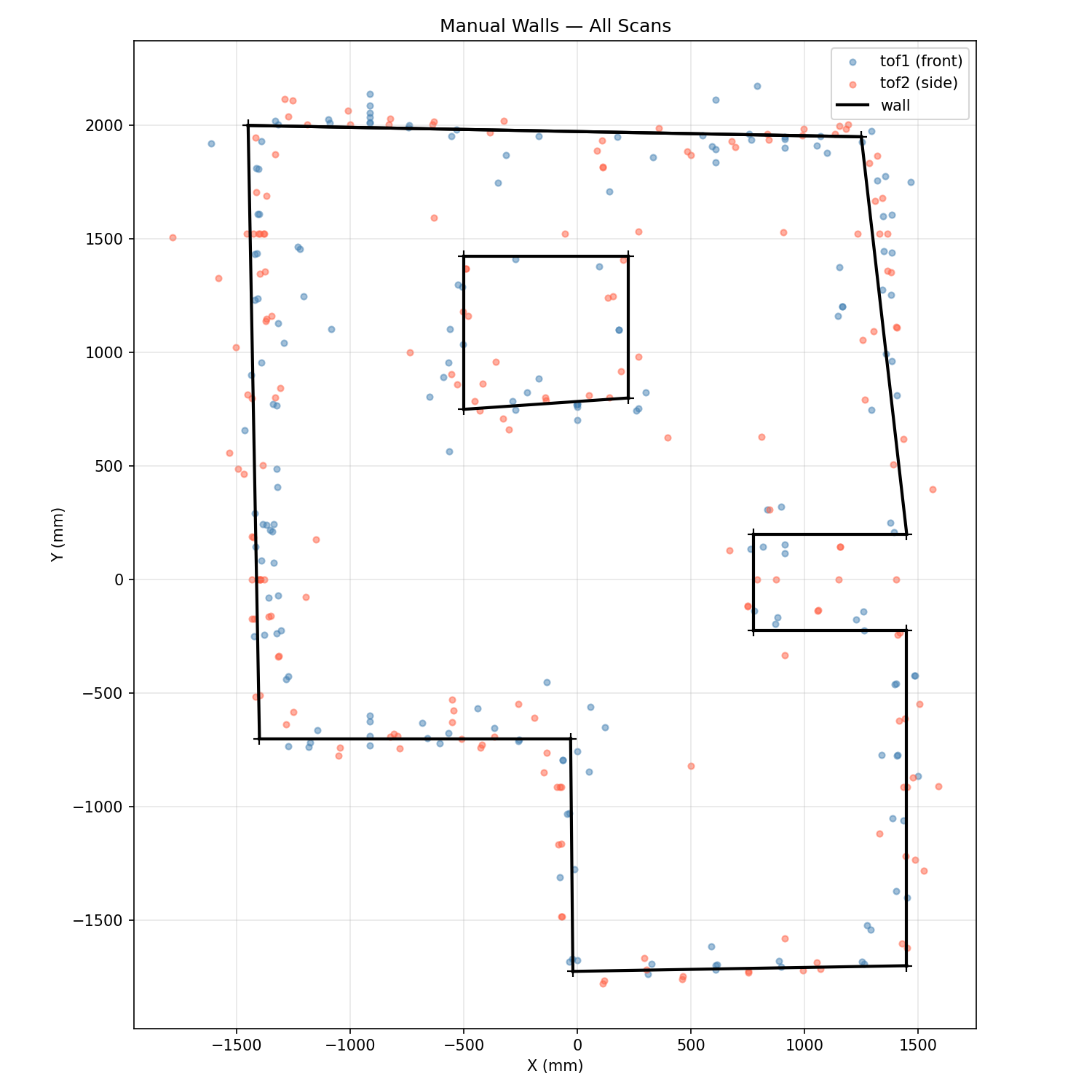
All five scans merged into a single world frame scatter plot, with tof1 in blue and tof2 in red. The result is consistent with the known lab geometry, with some outliers near corners where the sensor beam clipped edges rather than flat wall surfaces.

Map with Wall Segments
Wall segments were fitted manually to the scatter data. Minor endpoint adjustments were made where slight heading offsets at individual scan positions produced small rotational shifts in the point clusters, likely from the robot not being placed perfectly parallel to the room axes at each scan start.
Accuracy
RPID kept per-step angular error within 2 degrees, and since the integrator resets each call, drift does not accumulate over the rotation. The dominant error source was ToF noise at longer ranges, reduced by averaging 4 readings per step. An additional source of error is that the left wheels require higher PWM than the right to overcome static friction, causing the car to drift slightly off the scan point during each rotation rather than turning purely on axis. This effect worsens as the battery loses charge, introducing a systematic positional offset between readings that the transformation matrices cannot correct.
References
I used AI assistance to help structure the write-up and check syntax.